Introduction
In this assignments, you will get to practice what you have learned about LibreOffice calc, and also learn a few new things. Let's get started!
Jugaad Hardware & Tools
Jugaad Hardware & Tools is a hardware shop in your locality. Now that you have learned LibreOffice Calc, you have decided to digitize their inventory management, which has been done manually till now. As they have grown a lot over the past year, manually managing this data has become tedious and also a lot of calculations have to be done manually and repeatedly as new items get delivered and existing items are sold (stock movement or transactions). CS17 student to the rescue!
Basic data entry has already been done in a spreadsheet file. Start by downloading that file using this link.
The Sheets
Open the downloaded file. It has a total of 5 sheets:
- Item_Master: A list of all the different items they buy/sell.
- Suppliers: These are the entities/businesses from which Jugaad Hardware purchases or procures these items.
- Stock_Transactions: Every stock movement that happens. For example, they sell 5 fevicol boxes, the transaction will be of type "OUT" meaning stock moved out of their store.
- Current_Stock: This sheet is mostly empty and will contain the stock levels of different items and related columns/fields.
- Dashboard: Will contain an overview of their inventory with basic summary.
Basics
None of the sheets have any header/title yet. Your first task is to add nicely formatted headers. Let's start with the Item_Master sheet:
- Add 2 new rows at the top of the Item_Master sheet
- Merge the cells: C1, C2, D1, D2
- Add the title: "Items: Jugaad Hardware & Tools"
- Format as below:
- Black background
- Font should be white and 16pt
- Center Aligned both horizontally and vertically
Hint for centring vertically
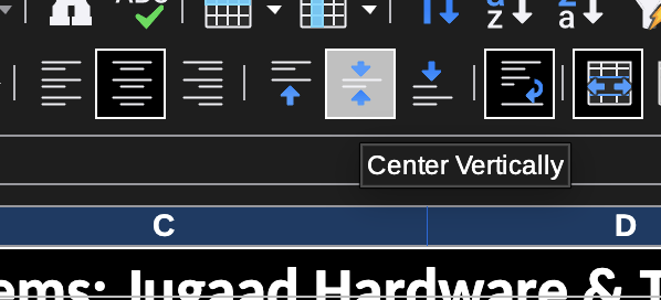
Now do the same for other sheets too. Replace "Items" with relevant name: "Dashboard", "Supplier", "Current Stock", and "Stock Transactions".
Current Stock Sheet
This sheet already has the Item ID column, look up and fill these columns from Item_Master sheet:
- Item Name
- Category
- Opening Stock
- Unit Cost
- Reorder Level
SUMIF
We have already learned about COUNTIF, which counts the number of rows where a particular condition is satisfied or TRUE. There is another similar function named SUMIF which will add (sum) the values instead of counting them.
Here is an example:
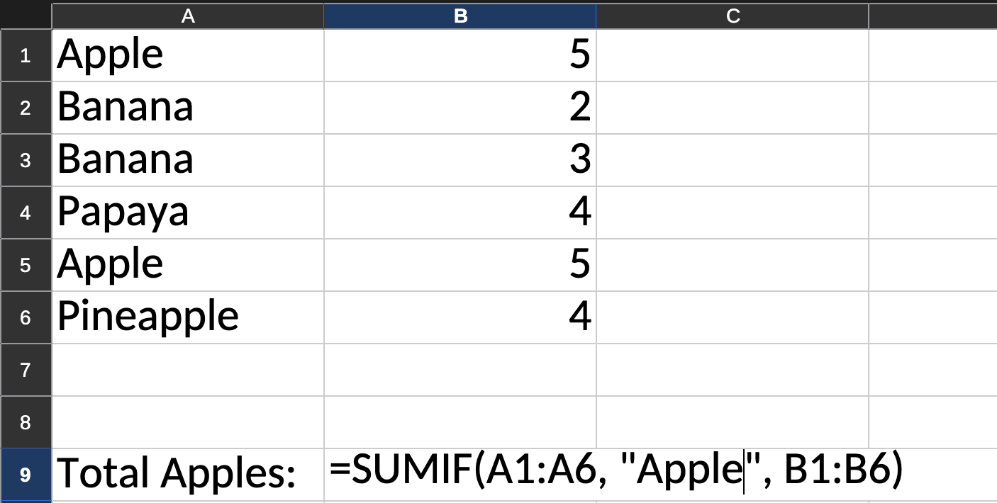
- First you give the range in which you want to apply the condition:
A1:A6 - Second is the condition, in this case it is which cells are equal to
"Apple" - Third is which column / range to sum / add, in this case we want to add the values in the B column, hence
B1:B6
Once you hit enter, you will see the answer comes out to be 10, which is correct. It adds B1 and B6 (rows where value of A column is "Apple"). SUM adds everything in the range, but SUMIF gives you power to add rows based on some condition of a particular column.
SUMIFS & COUNTIFS
Both COUNTIF and SUMIF take a single condition, but there are variants of this function which can take multiple conditions and only return TRUE when all the conditions are TRUE, here are examples:
=COUNTIFS(A1:A6, "Apple", B1:B6, ">5")
Here we are applying two conditions, one on column A value should be equal to "Apple" AND column B value should be greater than 5.
Similarly, there is SUMIFS :
=SUMIFS(B1:B6, A1:A6, "Apple", C1:C6, "In Stock")
The above will add the values of column B, where value of column A is "Apple" and values of column C is "In Stock". Notice the difference, in SUMIF you had the condition first, here we have the range to sum first. You can add as many range-condition pairs here:
=COUNTIFS(range1, condition1, range2, condition2, range3, condition3, ....)
=SUMIFS(range_to_sum, range1, condition1, range2, condition2, ...)
Current Stock Phase 2
Now that you know about SUMIFS, use your new found knowledge to implement the below columns in the Current_Stock sheet:
- Total Purchased — sum of
QuantitywhereType= "IN" for this Item ID - Total Sold, Damaged Qty, Returned Qty — same pattern as Total Purchased over types OUT, DAMAGE, RETURN.
- Current Stock — compute as Opening Stock + Total Purchased − Total Sold − Damaged Qty + Returned Qty
- Stock Value — Current Stock × Unit Cost
IF & IFS
The IF function let's you take a conditional and output a value if the expression evaluates to TRUE and another value if it evaluates to FALSE. Here is the example usage:
=IF(10>12, "yes", "nope") # will show "nope" in the cell
=IF(15>12, "yes", "nope") # will show "yes" in the cell
=IF(TRUE, "yes", "nope")   # will show "yes" always
=IF(FALSE, "yes", "nope")   # will show "nope" always
=IF(D2="OUT", "Sale", "Purchase") # if cell D2 is equal to OUT, Sales else Purchase
Just like SUMIFS and COUNTIFS allow you to add multiple conditions, IFS also lets us do the same:
=IFS(A2>=80, "A", A2>=60, "B", A2>=40, "C")
In the above example, the cell will show:
- A if
A2>=80 - B if
A2>=60 - C if
A2>=40 #N/Aif no condition matches
To tackle the case when no condition matches, we can add an always TRUE condition:
=IFS(A2>=80, "A", A2>=60, "B", A2>=40, "C", TRUE, "Fail")
Now the cell will show Fail if none of the first three condition match.
Application of IFS
Cool, enough with new functions now, let's use them to calculate Stock Status column in the Current_Stock sheet. Stock Status should be shown as follows:
- "Out of Stock" if Current Stock ≤ 0
- "Reorder" if Current Stock ≤ Reorder Level
- "OK" otherwise
Use IFS just like we did in last example of the previous section.
Conditional Formatting
Formatting cells based on certain conditions on the values of the cell makes it easier to makes sense of a long list of data. A user can easily peek and see what cells to pay attention to.
Format the Stock Status column to be of style:
- Error if it is "Out of Stock"
- Warning if it is "Reorder"
- Good if it is "OK"
After seeing the above formatting, Jaggu Uncle of Jugaad Hardware has requested you to add a Data Bar conditional formatting to the Stock Value column, so he can easily see which items are taking the most capital (money).
Dashboard
A dashboard is a single screen that shows you the most important numbers about your business at a glance. These numbers generally are statistics like total, average, etc. Dashboards also commonly have nice charts.
BTW quick tip before we proceed for the tasks, you can use the merge cells button from the toolbar to quickly select and merge required cells:
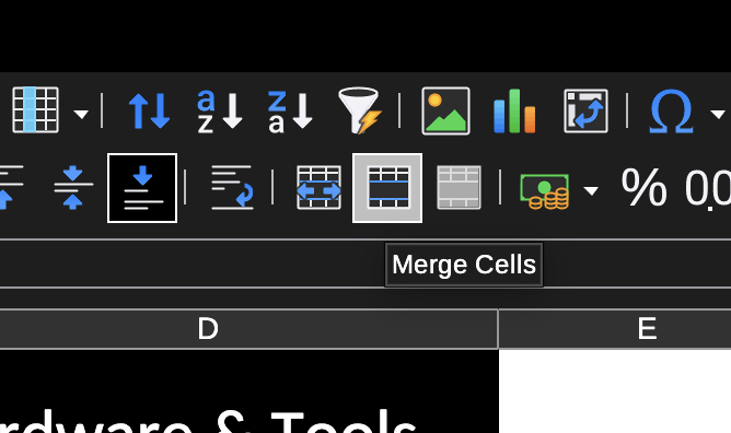
Add the following values (USE FORMULAs for NUMBERS!) to the dashboard in the cells and styles mentioned below:
- "Total Items" (B4) - Style with Accent 3
- The value will be the count of all items in the
Item_Mastersheet (hint: useCOUNTA) - B5 and B6 will be merged for this
- Style with Heading 1
- Align the value centre horizontally and vertically
- "Total Stock Value" - Style with Accent 3, should be in cells D4 and E4
- The value will be the sum of all stock value in
Current_Stocksheet - Cells D5:E6 will be merged for this
- Align the value centre horizontally and vertically
- Style with Heading 1
- Format as INR currency
- "Items to reorder" - Style with Accent 3, should be in B10
- The value will be in B11 and is the count of items that are needed to be re-ordered
- Style to be used is Neutral
- "Out of stock" - Style with Accent 3, should be in C10
- The value will be in C11 and is the count of items that are out of stock
- Style to be used is Error
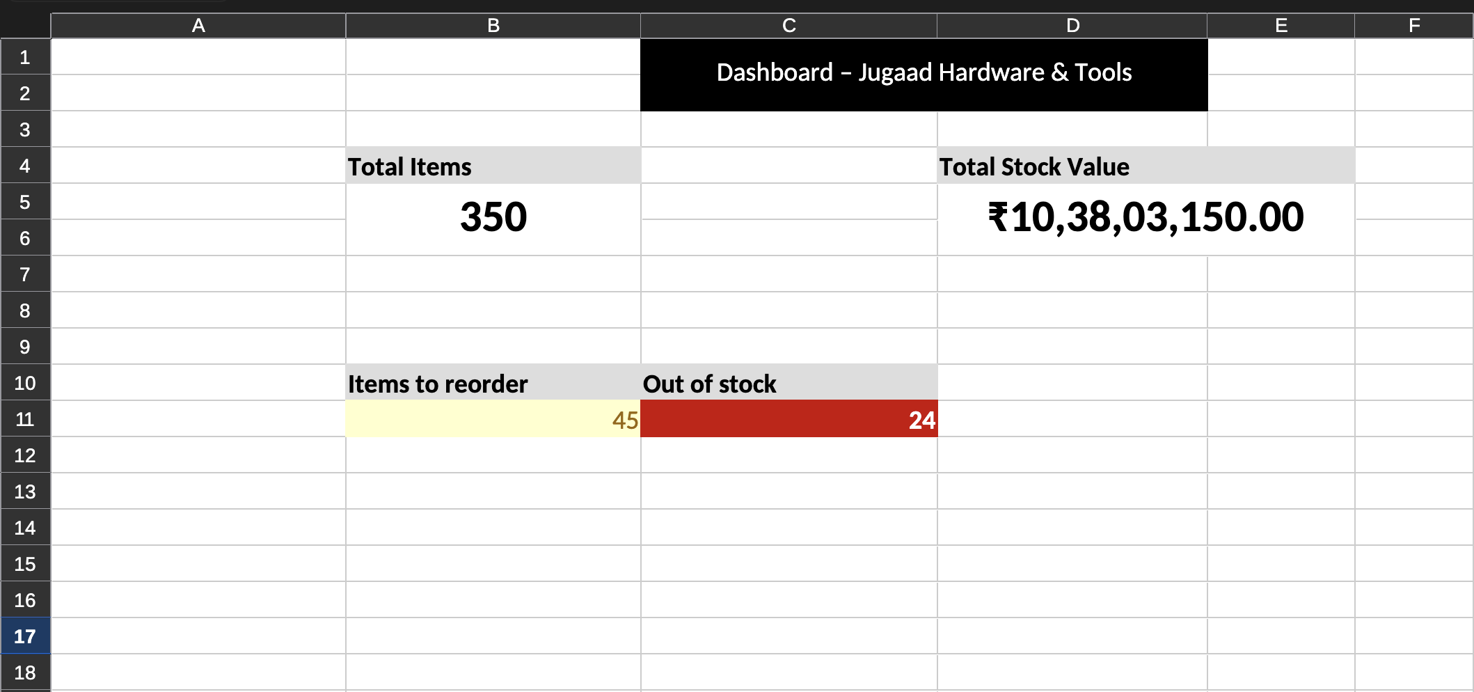
Here is how the completed dashboard sheet should look like:
Submission
Rename the file to <your_first_name>_jugaad_inventory.odt and send it to hussain@cs17.org.